INTERACTIVE MODELS IN TEACHING AND LEARNING

Example: MathKit models in a standard lesson

Classical Definition of Probability

Equipment

• Projector+ laptop
• Computer lab (for self-study)

Goals of the lesson

1. To get to know the classical definition of probability.
2. To build up the ability to construct mathematical models of random experiments.
3. To develop the skills of computing probabilities of random events in real-life setting.
4. To enhance the understanding of the laws inherent to random events.

Structure of the lesson

SECTION 1

Topic 1

Goals of the topic

• To remind students of the statistical definition of probability as the limit of relative frequency;
• By means of a computer experiment, to demonstrate the convergence of frequencies as the number of trials grows;
• To pose the problem of theoretical prediction of the frequency limit without actual experiments.

Form of work

• Demonstration of the model via projector;
• Group discussion.

Possible scenario

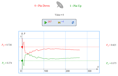
	Recall that the probability of a random event was defined as the number to which the relative frequency of this event converges as the number of trials grows. Consider a thumbtack tossing experiment. It can end in two ways: the tack can fall on the floor sharp point up or sharp point down. Can anybody predict the probability of each of these outcomes?
	No, to estimate this probability we must run a series of tossing experiments, calculate the frequencies of both outcomes, and evaluate the numbers which they approach.
	Can we say anything about the sum of these probabilities?
	Yes, it is equal to 1.
	Let us conduct the experiment with the tack in our virtual lab. Tack tossing experiment Can you evaluate these probabilities now, even if approximately?
	Yes. The probabilities can be estimated based on the frequencies thus obtained. We can increase the number of experiments to obtain a more precise estimate.

Notes for a teacher

Discussing this model, the teacher can make two important remarks:

• probability is inherent in “the nature of things:” if an experiment, say the one with the tack, is repeated a week later, the frequency will tend to the same number (for a tack made in a technologically different way this number can be different);
• considerable deviations of the relative frequency from the probability are possible even after a great number of trials; but the greater is this number, the less probable are such deviations (the question of quantitative estimation falls beyond the scope of school curriculum).

Topic 2

Goals of the topic

• To introduce a simple experiment in which the probabilities of outcomes can be predicted without running the experiment itself.

Form of work

• Demonstration of the model via projector;
• Group discussion.

Possible scenario

	In some cases the probability (i.e., the future frequency) can be predicted without running the experiment itself. Can you give examples of such experiments?
	Yes. For instance, tossing a coin, dice, the game of roulette, etc.
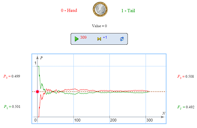
	Consider the coin tossing experiment. What is the probability to get heads in one tossing?
	1/2
	Why?
	A coin is symmetric. It has two sides. Hence, the experiment has two equally possible outcomes.
	Let’s check the answer experimentally. Tossing a coin

Notes for a teacher

Some students may doubt the symmetry of a coin because it has different engravings on its sides. However, this difference is so insignificant that an ideal coin, whose both sides are equally probable, can serve an absolutely adequate model of a real coin.

Topic 3

Goals of the topic

• To demonstrate an experiment with equally likely outcomes;
• To bring students to the understanding of that classical approach to the calculation of probability.

Form of work

• Demonstration of the model via projector;
• Group discussion.

Possible scenario

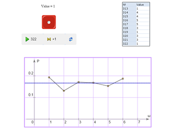
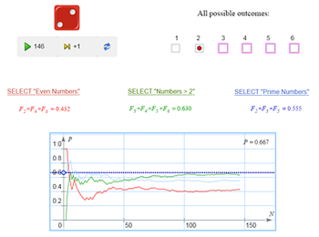
	Consider a die rolling experiment. Find the probability that the die shows five points.
	1/6
	Why?
	A die is symmetric. It has six faces.
	Let’s run this experiment. Rolling a die (Outcomes) The varying diagram seen on the screen is what is called the frequency polygon. As the number of trials grows, the diagram changes and in so doing shows how the frequencies of all the six outcomes gradually even out.
	How to find the probabilities of random events that consist of several rather than just one outcomes in such an experiment with equiprobable outcomes? Try to answer the following questions: What is the probability to obtain an even number? A number greater than 2? A prime number? Explain your answers. We’ll check each answer using our model. Rolling a die (Outcomes) The varying diagram seen on the screen is what is called the frequency polygon. As the number of trials grows, the diagram changes and in so doing shows how the frequencies of all the six outcomes gradually even out.
	Correct answers: 1/2; 2/3; 1/2.

Notes for a teacher

Explaining the answers, students are expected to arrive themselves at the classical definition of probability, which is formulated in the following conclusion.

Conclusion

	In our examples with a coin and a die we dealt with symmetric objects; therefore, all outcomes were equally likely. When a coin is tossed we have two equally likely outcomes: head and tail, and in rolling a die, six (the number of its faces). By the symmetry, we had no grounds to consider any of these outcomes more probable than another. In the general case, the following definition can be given (it’s called the classical definition of probability): Definition. Suppose that a random experiment can end in any of n equally likely outcomes; and suppose that exactly m of these outcomes are favorable for a random event A (i.e., they entail that A occurs). Then the probability of this event can be found by the formula P(A) = m / n Can we use this definition in the experiment with a tack?
	No, it’s not symmetric. The outcomes are not equally likely.
	To use this definition, we must determine all possible outcomes of the experiment; make sure they are equally likely; find the number n of all possible outcomes of the experiment; find the number m of the outcomes favorable for the given event A; compute P(A) = m / n.

Notes for a teacher

Stress the importance of step 2: if a mistake was made at this step (the outcomes you’ve chosen were not equally likely), then the other steps become meaningless.

SECTION 2

At this stage of the lesson the newly given definition is applied to the calculation of probabilities of random events in more involved experiments.

Example 1

Goals of the example

• To consider the simplest experiment in which elementary outcomes are combinations;
• To show that outcomes can be chosen in different ways and may turn out to be equally likely or not, depending on their choice.

Form of work

• Demonstration of the model via projector;
• Group discussion.

Possible scenario

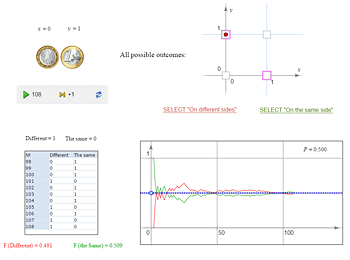
	We roll two coins. How many different outcomes does this experiment have? Name them.
	Correct answer: 4 (HH, HT, TH, TT)
	What is the probability that the coins show different sides? The same side? Explain your answers.
	Correct solution: the total number of outcomes is 4; the number of favorable ones for both questions is 2; so in both cases the probability is 1/2. Wrong solution: the total number of outcomes is 3; the numbers of favorable outcomes are 1 and 2 respectively; the corresponding probabilities are 1/3 and 2/3.
	Let’s check which of the two solutions is correct experimentally: Two coins Assuming that the experiment has four equally likely outcomes shown in the figure at right top, we find out that each of the events in question has two favorable outcomes; therefore, their probabilities are 1/2 each. This is confirmed by the frequencies’ behavior.

Notes for a teacher

If, having been asked about the number of outcomes, all students unanimously give the correct answer, four, the teacher can accept the wrong point of view and come up with three outcomes (this is the “D’Alembert error,” which he made in one of his arguments on probabilities).

Example 2

Goals of the example

• To consider an experiment in which elementary outcomes are number pairs;
• To demonstrate a visual technique of counting favorable outcomes by means of a table.

Form of work

• Demonstration of the model via projector;
• Group discussion;
• Work at the class board.

Possible scenario

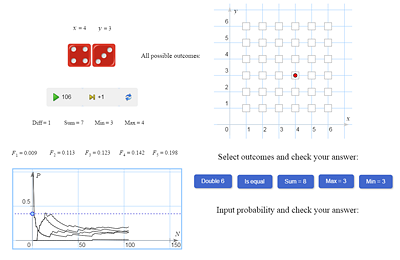
	We roll two dice. How many equally likely outcomes does this experiment have? What are they?
	36 outcomes. These are all possible pairs of numbers from one to six.
	Such pairs can be represented by the squares of the 6×6 table in the model. Let’s use it to find all favorable outcomes for each of the following events: A = {double six}, B = {same numbers}, C = {the sum of points on both dice is 8}, D = {the greater number is 3}, E = {the smaller number is 3}. Two dice (Outcomes & Events)
	A student comes to the class board and tries to answer the questions using the model. Correct answers: 1; 6; 5; 5; 7.
	Now it’s not difficult find the probabilities of all the events described above.
	Answers: 1/36; 1/6; 5/36; 5/36; 7/36;
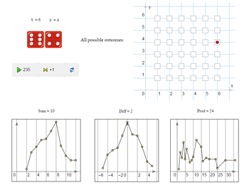
	And now, using the same model, let’s try to answer the following questions: What value of the sum is the most probable? What value of the difference is the most probable? What value of the smallest number is the most probable? What value of the greatest number is the most probable? What value of the product is the most probable? To check the answers, we use the same model: Two dice (Random Values)
	A student comes to the class board and tries to answer the questions using the model. All the answers are checked experimentally. Correct answers: 7; 0; 1; 6; 6 and 12.

Notes for a teacher

The example lays grounds for the subsequent introduction of the notion of random variable, the central notion in the second half of the probability course. Essentially, in the last activity the distribution laws of the random variables Sum, Diff, Min, Max, and Prod are studied.

Example 3

Goals of the example

• To consider a complex experiment in which simple random sampling without replacement (or simultaneous sampling) emerges for the first time as the drawing of two balls from a container (an “urn”);
• To discuss the “elementarity” of outcomes as one of the conditions for them to be equally possible.

Form of work

• Demonstration of the model via projector;
• Group discussion.

Possible scenario

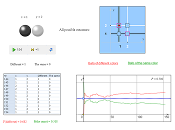
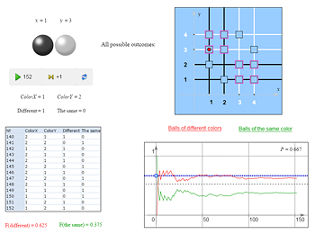
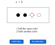
	Two balls are drawn from an urn with 2 white and 2 black balls. Find the probability that they are of different colors?
	Possible wrong answers: 1/2, 1/4, 1/3. The correct answer, 2/3, usually, is the rarest.
	Let’s start with the answer 1/2. Apparently, the students who suggest it have in mind the following model, which we met in the two-coin experiment: Two white and two black balls (A wrong model) But in our current experiment this model doesn’t work! To make sure of that, let’s launch a series of trials. We see that the four outcomes in question are not equiprobable. Can you explain why the outcomes WW and BB are much less frequent?
	???
	Here is a possible explanation: the outcomes we've chosen are NOT elementary, and therefore, they are not equally likely. The nature distinguishes balls rather than their colors. Imagine that there are two white and two million black balls. Then the likelihood of our outcomes is obviously different. Can you say what outcome shall we almost surely obtain in our experiment in the last case?
	Of course, BB.
	And now let’s look at the correct model. Two white and two black balls (The correct model) If we number all the balls and draw them one after another, then the experiment, as the table shows, will have 16 – 4 = 12 equiprobable outcomes (four pairs with equal numbers are excluded). Let’s assume that balls 1 and 2 are black and balls 3 and 4 are white. Then it is easy to single out all the outcomes favorable to our event and make sure that there are 8 of them. Answer: the probability that the balls will be of different color is 8/12 = 2/3.
	The same answer can be obtained much faster by the following simple argument: Let’s draw the first ball. Whatever color it is, there are three balls remaining in the box only one of which is the same color and the two others are of the other color. It follows that the probability to draw a ball of color different from that of the first ball is 2/3. This method can be also illustrated by a model: Two white and two black balls (Another model)

Notes for a teacher

1. If the correct answer, 2/3, is given straight away and no other answers are suggested, the simpleton’s part can be played by the teacher. Then the explanation of wrong answers can be as follows:

   • 1/2, for the set of outcomes {WW, WB, BW, BB};
   • 1/3 for the set of outcomes {WW, WB, BB} (here WB and BW are identified, because the balls are drawn simultaneously);
   • 1/4: we extract ne of four balls, that’s why this probability (however strange, such an explanation can be heard, too).

2. In the construction of a “correct” model, we may disregard the order in which the balls are drawn (i.e., they are drawn simultaneously); then the number of equiprobable outcomes reduces from 12 to 6. But the number of favorable outcomes also reduces by half, and so the answer remains the same, 4/6 = 2/3.

Game

Goals of the game

• To show practical benefits of the classical definition of probability in estimating the chances to win a game;
• To discuss an important property of mathematical relations, that of transitivity.

Form of work

• Playing a game with the class using the computer model;
• Group discussion of the results.

Possible scenario

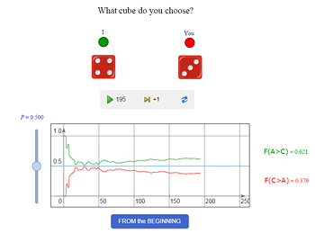
	We have three unusual (but “regular”) dice with the following numbers on their faces: die A: 1,4,4,4,4,4 die B: 2,2,2,5,5,5 die C: 3,3,3,3,3,6 You can choose any of the dice. After that I choose one of the other two dice and we roll them: if your number is greater than mine, you win and vice versa. Which of he dice will you choose?
	Possible answer: A (B, C).
	Then I choose (respectively) B (C, A). After one or even several games the “power” of a die will hardly show itself, so let’s run a long series of games and determine who wins more often. Game “Three dice” Students are allowed to change their choice. They loose again. Finally, the third, and last, attempt. And failure again.
	Let’s try to understand why the second player in all the three cases wins more often despite the first player’s advantage of choosing a more “powerful” die. If compare the dice with one another, it turns out that none of them is absolutely the “best.” The situation is similar to Russian kid’s game “Rock-Scissors-Paper”: the rock blunts scissors, scissors cut paper, and paper wraps the rock. Now, using the classical definition of probability and the computer model of the game, let us calculate and compare the probabilities of each of the following events: P(B>A) and P(A>B), P(C>B) and P(B>C), P(A>C) and P(C>A).
	A student comes to the class board and, with a help from the class and the model finds favorable outcomes, counts them, and computes the probabilities: P(B>A) = 21/36 and P(A>B) = 15/36, P(C>B) = 21/36 and P(B>C) = 15/36, P(A>C) = 25/36 and P(C>A) = 11/36.
	Thus, in two-player games, die B is better than die A, C is better than B, and A is better than C. This means that it’s better to be the second player and choose the die when the choice of the first player is known. And what about the same game for three players? What will your strategy be? Think about this problem at home. We’ll discuss your answers and run a computer experiment.

Notes for a teacher

1. The paradox we discovered is called the nontransitivity paradox. The point of the matter is in the fact that the relations expressed in our everyday life by the words “greater,” “better,” “stronger,” and so on are usually implied to be transitive: if A is better than В and B is better than C, then A is better than C. However, this far from always being the case: for example, the relation “greater than” for numbers is transitive, while the relation “stronger” for chess players based on the results of their games with one another isn’t.

2. Here is the answer to the last question: one must choose a die first and take die B. The probability that the greatest of the three numbers shows up on die A is 75/216, for die B it is 90/216, and for C, 51/216.

SECTION 3

Problems

Problem 1 (a)	(a) Small Varya has two pairs of mittens. When she goes out, she takes two mittens at random. Find the probability that they will be paired, i.e. for different hands: a left one and a right one?
Problem 1 (b)	(b) Imagine that in question (a) Varya has lost one mitten. She is going out again and chooses two mittens from three. The question remains the same: what is the probability that they turn out to be paired?
Problem 2	Ten persons throw lots to form two equal teams. Find the probability that Petya and Vasya will play for different teams? For the same team?
Problem 3	Three persons came to a restaurant wearing the same hats and left them in the coatroom. When they were leaving the restaurant, they put their hats on at random. What is the probability that each of them will leave in his own hat? That none of them will wear his own hat?
Problem 4	Car license number consists of three digits. Find the probability that a randomly chosen number will be symmetric?
Problem 5	Find the probability to obtain the same word after a random rearrangement of letters in the word (a) COME; (b) HIGH; (c) NOON.
Problem 6	There are four pairs of shoes in a closet of sizes 42 through 45. Two shoes are chosen from the closet at random. What is the probability that they make a pair (i.e. they are of the same size)?
Problem 7	There are four identical pairs of boots of 45th size in a closet. Two boots are chosen at random from them. What is the probability that they form a pair (i.e. one left and one right)?
Problem 8	A group of 5 tourists chooses by lot two of them to go to a neighboring village to buy some food. Paul doesn’t want to go, but he’ll obey the lot. Find the probability that Paul will have to go to the store.
Problem 9	Two pupils on duty are chosen by lot from Natasha’s class, which consists of 9 girls and 6 boys. Find the probability that (a) Natasha will be on duty; (b) Natasha and her friend Sveta will be on duty; (c) a boy and a girl will be on duty.